One-way ANOVA
This page is a hands-on run-through of a one-way ANOVA with jaov(): which version of the test to run, how to check the assumption that decides between the two versions, which follow-up comparisons go with each, and what to put in your write-up.
A one-way ANOVA (analysis of variance) compares the average of a numeric outcome across the categories of one categorical variable — usually three or more groups. The page assumes you have met the test in a course or a textbook, and concentrates on running the test and reporting it.
This page follows the pattern of every How-To: numbered blocks that build one script, with the finished script to download at the bottom. Using the How-To pages explains the pattern, and how to reset your session if something goes wrong.
1. Load jstats and choose the data
We’ll work on clinic, one of the two practice datasets that ship with the package: 70 simulated clients in a study of four treatment conditions — a control group, cognitive behavioral therapy (CBT), mindfulness training, and a support group. juse() makes clinic the default data frame, so the commands that follow can leave its name out.
## ---- 1. Load jstats and choose the data -------------------------------

## Load jstats for this session, then make the clinic practice dataset
## the default, so the commands below can leave its name out
library(jstats)
juse(clinic)
The command lines are shown; the standalone ## comment lines aren’t – running a comment just echoes it back and does nothing.
Console (lower-left pane)
ConsoleTerminal×Background Jobs×> library(jstats)
jstats v0.9.267 is up to date.
For jstats conventions (useful to AI assistants too), run jai().
> juse(clinic)
Default data frame set to: clinic
> |
2. Run the standard ANOVA
The outcome is Flourishing, a wellbeing score from 0 to 100, and the grouping variable is Condition. jaov() takes a formula, with the outcome on the left of the tilde (~) and the grouping variable on the right.
## ---- 2. Run the standard ANOVA ----------------------------------------

## Is there evidence that average flourishing differs across the four
## treatment conditions? The outcome goes left of the ~, the groups right
jaov(Flourishing ~ Condition)
Console (lower-left pane)
ConsoleTerminal×Background Jobs×> jaov(Flourishing ~ Condition)
One-Way ANOVA
Using default data frame: clinic

Analysis N: 70

Group Descriptives: Flourishing by Condition
Group              N   Mean     SD    95% CI Lower  95% CI Upper
----------------  --  ------  ------  ------------  ------------
1: Control        18  42.111  16.193     34.058        50.164
2: CBT            14  56.143  11.114     49.726        62.560
3: Mindfulness    17  55.353  12.232     49.064        61.642
4: Support group  21  47.000  11.167     41.917        52.083

ANOVA: Flourishing by Condition
Source     df  Sum of Squares  Mean Square    F      p
---------  --  --------------  -----------  -----  ----
Condition   3      2313.426      771.142    4.647  .005
Residual   66     10951.374      165.930
Total      69     13264.800

Eta-squared: 0.174

> |
The result is in the first row of the ANOVA table. The p is below .05, the usual threshold, so the test is statistically significant: evidence that average flourishing differs across the four conditions in the population from which the sample was selected, and not only in the sample.
TipIf you’re new to statistics
The four group means in the output differ; in real data they always do. That is not the question. These 70 clients are a sample, and the question is about the population from which the sample was selected: if the four conditions made no difference in that population, could differences this size have turned up in the sample simply through the luck of who was selected? The ANOVA is a test of exactly that. (With data on a whole population, a census, there would be nothing to test. The means you see would simply be the population’s means.)
NoteReading this output
- The title names the test. “One-Way ANOVA” is the standard version. The line under the title confirms which data frame was used, since the command left the data frame’s name out.
- Analysis N is the number of cases the test used — all 70 here, because neither variable has missing values. When cases are set aside, a small Case Processing table takes this line’s place and says how many and why (block 9 has one).
- Group Descriptives gives each group’s size, mean, and standard deviation, with a 95% confidence interval for the mean. Look here first: these are the differences in your sample.
- The ANOVA table is the test itself. Two numbers in its first row carry the result, F and p. The larger the F and the smaller the p, the stronger the evidence that the means differ in the population and not only in the sample. By the usual convention, a p below .05 counts as statistically significant. A significant result does not say the difference is large or important, and a non-significant result does not show the groups are the same in the population. The rest of the table, and the Eta-squared line under it, are covered in the books and in most statistics courses. You will need some of those numbers for a write-up; the last section of this page shows where to find them.
NoteWhy jstats does it this way
One function runs both versions of this test, the standard ANOVA and Welch’s ANOVA, and one argument, welch = TRUE, switches between them. The same argument does the same job in jstats’s t-test, jt(). Both functions default to the standard version, so a t-test and an ANOVA on the same two groups give the same answer.
Base R arranges things differently. Its standard ANOVA is aov(); Welch’s version is a separate function, oneway.test(), with different output. Base R’s t-test, t.test(), runs Welch’s version unless told otherwise, while aov() runs the standard version, so on the same two groups the two functions give different answers until you change a default. Levene’s test and the Games-Howell comparisons, both used later on this page, are not in base R at all. Add-on packages fill those gaps, each with its own syntax, defaults, and output.
Base R also has to be told that the grouping variable is categorical. Condition holds the codes 1 to 4 with labels attached, which is how data from commercial statistical software usually arrive. Hand Condition to aov() as it is, and R treats the codes as a measured quantity and runs a different analysis, with no warning. jaov() reads the labels, makes the conversion for you, and then runs base R’s own aov() underneath — the same proven code, with the setup done.
3. The other version, Welch’s ANOVA
jstats offers two versions of the test. The standard ANOVA you just ran assumes that the scores are about equally spread out in every group — equal variances, also called homogeneity of variance. Welch’s ANOVA drops that assumption.
The standard version is the default because it is the traditional one: the test most courses and textbooks teach, the table commercial statistical software prints first, and the one most readers of your work will expect unless you say otherwise. Welch’s version is one argument away: welch = TRUE.
## ---- 3. The other version, Welch's ANOVA ------------------------------

## The same question, without assuming the groups are equally spread out
jaov(Flourishing ~ Condition, welch = TRUE)
Console (lower-left pane)
ConsoleTerminal×Background Jobs×> jaov(Flourishing ~ Condition, welch = TRUE)
Welch's One-Way ANOVA
Using default data frame: clinic

Analysis N: 70

Group Descriptives: Flourishing by Condition
Group              N   Mean     SD    95% CI Lower  95% CI Upper
----------------  --  ------  ------  ------------  ------------
1: Control        18  42.111  16.193     34.058        50.164
2: CBT            14  56.143  11.114     49.726        62.560
3: Mindfulness    17  55.353  12.232     49.064        61.642
4: Support group  21  47.000  11.167     41.917        52.083

Welch's ANOVA: Flourishing by Condition
  F    df1   df2    p
-----  ---  ----  ----
4.232   3   35.1  .012

Note: Sum of Squares and Mean Square are not applicable to Welch's ANOVA.
For the standard ANOVA table, run jaov() without welch = TRUE.

Eta-squared: 0.174
(Note: Eta-squared is calculated from the traditional SS decomposition.)

> |
Welch’s ANOVA is significant too, so on these data the two versions lead to the same conclusion. The two versions will not always agree, and the next two blocks are about choosing between them.
NoteReading this output
The title now says Welch’s. The test table is shorter than the standard one: it shows F, two degrees-of-freedom values, and p, and the note under the table says that sums of squares and mean squares do not apply to Welch’s ANOVA. The second degrees-of-freedom value carries a decimal, which is normal for this test. F and p are read as in block 2. The Group Descriptives table is the same as in block 2, because Welch’s ANOVA changes how the means are tested, not the means. The Eta-squared line has a note of its own, because the effect size is still worked out the standard way.
NoteGoing deeper (optional)
Some statisticians now recommend running Welch’s version as a matter of routine, on the grounds that it costs little when the variances are equal and protects you when the variances are not. Others, and most courses, keep the standard test unless there is a reason to leave it. Either position is defensible. What matters is that you say which test you ran and why, and that you follow the preference of your field, or of whoever will assess your work, where there is one. The help page ?jaov documents every option used on this page; Book 1 covers what the F test is doing and why unequal variances matter, in more detail, with worked examples.
4. Check equal variances with Levene’s test
Whether the variances are equal is something you can check. Levene’s test compares the spread of the groups, and diagnostics = "levene" adds it to the output. Levene’s test is one of jstats’s diagnostics, checks on the assumptions behind an analysis, and the diagnostics stay off unless you ask for them. diagnostics = TRUE asks for all of them at once (for jaov(), Levene’s test and a normal Q-Q plot); this page asks for Levene’s test by name.
## ---- 4. Check equal variances with Levene's test ----------------------

## Levene's test asks whether the groups differ in spread. It is off by
## default, so ask for it by name
jaov(Flourishing ~ Condition, diagnostics = "levene")
Console (lower-left pane)
ConsoleTerminal×Background Jobs×> jaov(Flourishing ~ Condition, diagnostics = "levene")
One-Way ANOVA
Using default data frame: clinic

Analysis N: 70

Levene's Test for Homogeneity of Variance
  F    df1  df2    p
-----  ---  ---  ----
0.788   3    66  .505

Group Descriptives: Flourishing by Condition
Group              N   Mean     SD    95% CI Lower  95% CI Upper
----------------  --  ------  ------  ------------  ------------
1: Control        18  42.111  16.193     34.058        50.164
2: CBT            14  56.143  11.114     49.726        62.560
3: Mindfulness    17  55.353  12.232     49.064        61.642
4: Support group  21  47.000  11.167     41.917        52.083

ANOVA: Flourishing by Condition
Source     df  Sum of Squares  Mean Square    F      p
---------  --  --------------  -----------  -----  ----
Condition   3      2313.426      771.142    4.647  .005
Residual   66     10951.374      165.930
Total      69     13264.800

Eta-squared: 0.174

> |
Levene’s test is not significant here: its p is above .05. The test found no evidence that the four conditions differ in spread in the population, so there is no reason to doubt the standard ANOVA’s assumption, and the standard ANOVA from block 2 is the one to report.
Equal variances is the assumption most people have in mind when they talk about checking an ANOVA, and it is the assumption that decides between the two versions of the test. Both versions make two other assumptions as well: that the cases are independent of one another, and that the scores within each group are roughly normally distributed. The box plot in block 8 gives a first look at the second of those, and diagnostics = "qq" draws a normal Q-Q plot, a closer one.
NoteReading this output
The new table sits at the top, above the descriptives. Levene’s test has an F and a p of its own, and its p is read the other way around from most tests: a p above .05 is the reassuring result. When Levene’s test is not significant, jstats adds nothing further, and the rest of the output is what block 2 printed.
Glance at the SD column of Group Descriptives as well. Levene’s test is a guide, not a verdict: with small groups the test can miss a real difference in spread, and with very large groups the test can flag a trivial one. Here the Control group’s SD is the largest of the four, though not by enough for Levene’s test to flag it; block 8 shows where that extra spread comes from.
5. When Levene’s test is significant
To see the other outcome of Levene’s test we need a different variable. ScreenTime is each client’s daily screen time, in hours.
## ---- 5. When Levene's test is significant -----------------------------

## A different outcome, daily screen time, whose spread does differ
## across the conditions. Watch for the note under the Levene table
jaov(ScreenTime ~ Condition, diagnostics = "levene")
Console (lower-left pane)
ConsoleTerminal×Background Jobs×> jaov(ScreenTime ~ Condition, diagnostics = "levene")
One-Way ANOVA
Using default data frame: clinic

Analysis N: 70

Levene's Test for Homogeneity of Variance
  F    df1  df2    p
-----  ---  ---  ----
3.308   3    66  .025

Note: Levene's test is significant (p = .025).
The largest group is 1.5 times the smallest, and the largest standard deviation
is 2.1 times the smallest.
Guidelines differ on whether the standard ANOVA is acceptable at these values.
Welch's ANOVA does not assume equal variances: welch = TRUE.
See ?jaov.

Group Descriptives: ScreenTime by Condition
Group              N   Mean    SD   95% CI Lower  95% CI Upper
----------------  --  -----  -----  ------------  ------------
1: Control        18  4.128  1.151      3.555         4.700
2: CBT            14  4.107  2.463      2.685         5.529
3: Mindfulness    17  4.671  2.273      3.502         5.839
4: Support group  21  3.671  2.017      2.753         4.590

ANOVA: ScreenTime by Condition
Source     df  Sum of Squares  Mean Square    F      p
---------  --  --------------  -----------  -----  ----
Condition   3        9.382        3.127     0.778  .511
Residual   66      265.424        4.022
Total      69      274.806

Eta-squared: 0.034

> |
This time Levene’s test is significant: evidence that the four conditions differ in spread in the population. jstats adds a note under the Levene table. The note’s second sentence states the two things that decide how much unequal spread matters: how far apart the group sizes are, and how far apart the standard deviations are. Here the note says that guidelines differ on whether the standard ANOVA is acceptable, and points to Welch’s ANOVA.
That gives a rule for choosing between the two versions:
- Levene’s test not significant: report the standard ANOVA.
- Levene’s test significant, and the note says the standard ANOVA is usually still acceptable (group sizes and SDs both close): the standard ANOVA is a reasonable choice. Say which version you used.
- The note says guidelines differ, as here: Welch’s ANOVA is the safer choice.
- The note says the standard ANOVA’s p-value may not be reliable (group sizes and SDs both far apart): use Welch’s ANOVA.
The rule is a rule of thumb, not a guarantee, and textbooks draw its lines in different places. The help page ?jaov, in its section Unequal variances, gives the lines jstats draws and the sources behind them. Whichever version you choose, say what you did and why.
NoteReading this output
Levene’s p is below .05, and the SD column shows why: the Control group’s screen time is bunched more tightly than the other groups’.
The note’s second sentence gives two ratios. The first compares the largest group with the smallest: 21 clients against 14, which is 1.5. The second compares the largest standard deviation with the smallest: 2.463 (CBT) against 1.151 (Control), which is 2.1. Unequal spread matters least when the groups are about the same size and the SDs are not far apart, and most when both are far apart. These group sizes sit at the edge of one common guideline, a largest group no more than 1.5 times the smallest, and the SDs just past another, a largest SD no more than twice the smallest. So the note does not choose for you: it says that guidelines differ, and names the version of the test that does not assume equal variances.
The ANOVA itself is not significant in this output: the test gives no evidence that average screen time differs across the conditions in the population. Levene’s test and the ANOVA answer different questions, one about spread and one about means.
6. Which groups differ, Tukey HSD
Back to Flourishing. A significant ANOVA is evidence that the group means are not all the same in the population. A significant ANOVA does not say which groups differ. That is the job of post-hoc comparisons: every pair of groups compared, with the p-values adjusted so that making several comparisons at once does not inflate the chance of a false alarm. posthoc = TRUE adds the comparisons, and after the standard ANOVA the method is Tukey HSD (the letters stand for “honestly significant difference”).
## ---- 6. Which groups differ, Tukey HSD --------------------------------

## Post-hoc comparisons test every pair of groups. After the standard
## ANOVA, the method is Tukey HSD
jaov(Flourishing ~ Condition, posthoc = TRUE)
Console (lower-left pane)
ConsoleTerminal×Background Jobs×> jaov(Flourishing ~ Condition, posthoc = TRUE)
One-Way ANOVA
Using default data frame: clinic

Analysis N: 70

Group Descriptives: Flourishing by Condition
Group              N   Mean     SD    95% CI Lower  95% CI Upper
----------------  --  ------  ------  ------------  ------------
1: Control        18  42.111  16.193     34.058        50.164
2: CBT            14  56.143  11.114     49.726        62.560
3: Mindfulness    17  55.353  12.232     49.064        61.642
4: Support group  21  47.000  11.167     41.917        52.083

ANOVA: Flourishing by Condition
Source     df  Sum of Squares  Mean Square    F      p
---------  --  --------------  -----------  -----  ----
Condition   3      2313.426      771.142    4.647  .005
Residual   66     10951.374      165.930
Total      69     13264.800

Eta-squared: 0.174

Tukey HSD Post-Hoc Comparisons
Comparison                 Mean Difference  95% CI Lower  95% CI Upper  p (adjusted)
-------------------------  ---------------  ------------  ------------  ------------
CBT-Control                     14.032           1.933       26.130         .017
Mindfulness-Control             13.242           1.759       24.724         .017
Support group-Control            4.889          -6.017       15.794         .641
Mindfulness-CBT                 -0.790         -13.043       11.463         .998
Support group-CBT               -9.143         -20.857        2.572         .178
Support group-Mindfulness       -8.353         -19.430        2.724         .203

> |
Two of the six comparisons are significant: clients in CBT and clients in Mindfulness each scored higher on flourishing than clients in the Control group. None of the other four comparisons reaches significance, CBT against Mindfulness included.
NoteReading this output
The new table is at the bottom. Each row is one pair of groups, and the row’s name says which way the subtraction runs: CBT-Control is the CBT mean minus the Control mean, so a positive difference means CBT scored higher. Next comes the 95% confidence interval for that difference, and then the adjusted p. Because the adjustment is built in, you read each p against .05 as it stands. The interval tells the same story: an interval that does not include zero goes with a p below .05.
Four groups make six pairs, and five groups would make ten, so this table grows quickly. If the table’s lines wrap in your Console, drag the Console pane wider and run the line again.
7. Which groups differ after Welch’s, Games-Howell
Tukey HSD carries the same equal-variances assumption as the standard ANOVA. If you used Welch’s ANOVA, the matching method is Games-Howell, which does not assume equal variances either. You don’t ask for Games-Howell by name: posthoc = TRUE gives Tukey HSD after the standard ANOVA and Games-Howell after Welch’s ANOVA.
## ---- 7. Which groups differ after Welch's, Games-Howell ---------------

## The same request after Welch's ANOVA gives Games-Howell comparisons,
## which do not assume equal variances either
jaov(Flourishing ~ Condition, welch = TRUE, posthoc = TRUE)
Console (lower-left pane)
ConsoleTerminal×Background Jobs×> jaov(Flourishing ~ Condition, welch = TRUE, posthoc = TRUE)
Welch's One-Way ANOVA
Using default data frame: clinic

Analysis N: 70

Group Descriptives: Flourishing by Condition
Group              N   Mean     SD    95% CI Lower  95% CI Upper
----------------  --  ------  ------  ------------  ------------
1: Control        18  42.111  16.193     34.058        50.164
2: CBT            14  56.143  11.114     49.726        62.560
3: Mindfulness    17  55.353  12.232     49.064        61.642
4: Support group  21  47.000  11.167     41.917        52.083

Welch's ANOVA: Flourishing by Condition
  F    df1   df2    p
-----  ---  ----  ----
4.232   3   35.1  .012

Note: Sum of Squares and Mean Square are not applicable to Welch's ANOVA.
For the standard ANOVA table, run jaov() without welch = TRUE.

Eta-squared: 0.174
(Note: Eta-squared is calculated from the traditional SS decomposition.)

Games-Howell Post-Hoc Comparisons
Comparison                 Mean Difference  95% CI Lower  95% CI Upper   df   p (adjusted)
-------------------------  ---------------  ------------  ------------  ----  ------------
CBT-Control                     14.032           0.871       27.192     29.6      .033
Mindfulness-Control             13.242           0.134       26.350     31.5      .047
Support group-Control            4.889          -7.436       17.214     29.5      .704
Mindfulness-CBT                 -0.790         -12.235       10.655     28.7      .998
Support group-CBT               -9.143         -19.630        1.344     28.1      .104
Support group-Mindfulness       -8.353         -18.739        2.034     32.9      .151

> |
The conclusion is the same on these data: the same two comparisons are significant, with somewhat larger p-values. Where the groups’ variances really do differ, the two methods can disagree, which is the reason to match the post-hoc method to the test.
NoteReading this output
The table has the same layout as the Tukey HSD table, with one more column, df. Games-Howell judges each pair on those two groups’ own variances, so each comparison has a degrees-of-freedom value of its own. You need the df column only if your write-up reports it. The mean differences are the same as in the Tukey HSD table, because they are simply differences between group means. The intervals and, as a rule, the p-values are not the same.
One caution. Games-Howell has to estimate each group’s variance from that group alone, and with very small groups its p-values can come out too small. A rule of thumb you will see quoted is at least six cases in every group.
8. Look at the groups with jplot()
A table of means summarizes each group in a few numbers; a plot shows what the numbers are summarizing. Save the ANOVA’s result under a name with the assignment operator, <-, and hand that name to jplot().
## ---- 8. Look at the groups with jplot() -------------------------------

## Save the result under a name, then hand it to jplot() for a box plot
## of each group. The plot appears in the Plots tab (lower-right pane)
Results <- jaov(Flourishing ~ Condition)
jplot(Results)
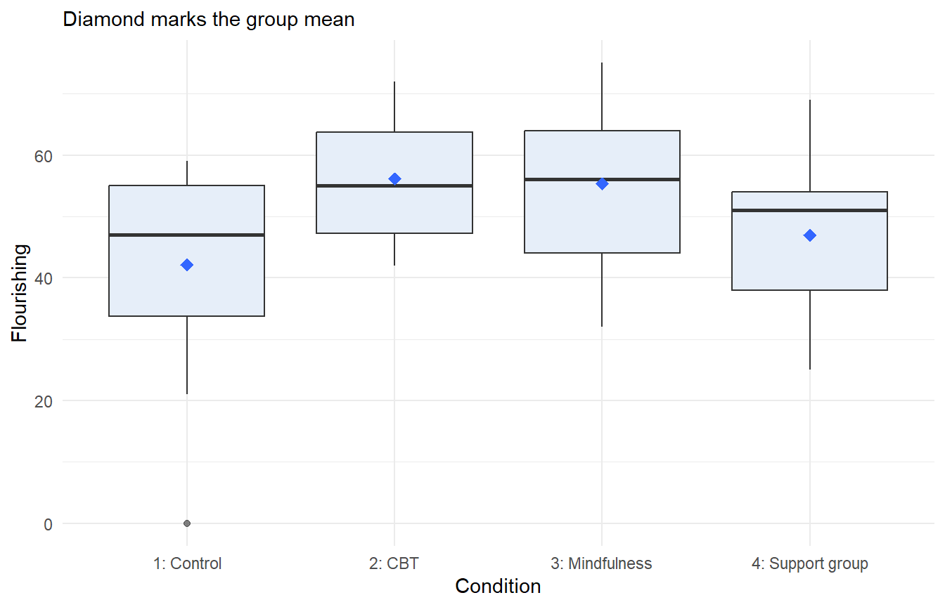
The first line prints the same output as block 2 while saving the result as Results. The second line draws a box plot of each group in the Plots tab of the lower-right pane:
One thing stands out: a single client in the Control group, far below everyone else, with a flourishing score of 0. A score like that deserves a look at the data before you rely on the result — is the score real, or a typing slip? (In these practice data the score is simply very low.)
NoteReading this output
Each box spans the middle half of that group’s scores, the heavy line across the box is the median, and the diamond marks the mean — the number the ANOVA compares. The lines above and below the box reach to the lowest and highest scores that are not unusually far from the box, and any score beyond those lines is drawn as a separate point. The horizontal axis labels each condition with its code and its name, as the Group Descriptives table does.
Two things are worth looking for, because either can distort a mean and a standard deviation. Skew: a median line well off the center of its box, or a diamond some distance from the median line, means the scores are stretched out in one direction. Outliers: the separate points. The Control client with a score of 0 drags the Control group’s mean down and stretches the Control group’s standard deviation; that one client is the main reason Control’s SD is the largest in the Group Descriptives table.
9. A group with one case
Sometimes a category turns up with a single case in it: one respondent who checked “Other,” one site that recruited one participant. It is worth knowing what each version of the test does then. No group in clinic is that small, so this block makes one. The subset = argument keeps only some of the cases, for this one call, and the rule written here keeps every client who is not in CBT, plus one client who is.
## ---- 9. A group with one case -----------------------------------------

## No group in clinic is that small, so make one for this call only:
## subset = keeps every client who is not in CBT (condition 2), plus one
## who is (!= means "is not equal to", and | means "or")
jaov(Flourishing ~ Condition, posthoc = TRUE,
     subset = Condition != 2 | ClientID == "C016")
Console (lower-left pane)
ConsoleTerminal×Background Jobs×> jaov(Flourishing ~ Condition, posthoc = TRUE,
+      subset = Condition != 2 | ClientID == "C016")
One-Way ANOVA
Using default data frame: clinic

Case Processing  Excluded  Remaining
    Original           --         70
    subset =           13         57  Condition != 2 | ClientID == "C016"
    Analysis N         --         57
-------------------------------------------------------------------------

Group Descriptives: Flourishing by Condition
Group              N   Mean     SD    95% CI Lower  95% CI Upper
----------------  --  ------  ------  ------------  ------------
1: Control        18  42.111  16.193     34.058        50.164
2: CBT             1  48.000
3: Mindfulness    17  55.353  12.232     49.064        61.642
4: Support group  21  47.000  11.167     41.917        52.083

ANOVA: Flourishing by Condition
Source     df  Sum of Squares  Mean Square    F      p
---------  --  --------------  -----------  -----  ----
Condition   3      1564.270      521.423    2.957  .041
Residual   53      9345.660      176.333
Total      56     10909.930

Eta-squared: 0.143

Tukey HSD Post-Hoc Comparisons
Comparison                 Mean Difference  95% CI Lower  95% CI Upper  p (adjusted)
-------------------------  ---------------  ------------  ------------  ------------
CBT-Control                      5.889         -30.298       42.076          .973
Mindfulness-Control             13.242           1.330       25.154          .024
Support group-Control            4.889          -6.425       16.203          .663
Mindfulness-CBT                  7.353         -28.890       43.596          .949
Support group-CBT               -1.000         -37.051       35.051         1.000
Support group-Mindfulness       -8.353         -19.844        3.138          .229

> |
The standard ANOVA still runs when a group has one case. But the test learns very little about that group, as the wide intervals on the CBT rows of the Tukey HSD table show.
NoteReading this output
A Case Processing table has replaced the one-line N at the top. The table reports that the subset = rule set aside 13 clients and left 57.
In Group Descriptives, the CBT row shows an N of 1 and a mean (that one client’s score) and then nothing. One case has no standard deviation, so the CBT row has no confidence interval either. The standard ANOVA can still run because it estimates the spread from the other three groups and applies that estimate to all four. In the Tukey HSD table, the three rows that involve CBT have intervals far wider than the other rows.
10. One case under Welch’s ANOVA
Welch’s ANOVA cannot do the same. Welch’s ANOVA needs each group’s own variance, and a single case does not have one. Run the same analysis as a Welch’s ANOVA and jstats stops — the one deliberate error on this page.
## ---- 10. One case under Welch's ANOVA ---------------------------------

## The same cases as a Welch's ANOVA. It needs each group's own variance,
## and one case has none, so jstats stops and says so
jaov(Flourishing ~ Condition, welch = TRUE,  # an error, on purpose
     subset = Condition != 2 | ClientID == "C016")
Console (lower-left pane)
ConsoleTerminal×Background Jobs×> jaov(Flourishing ~ Condition, welch = TRUE,  # an error, on purpose
+      subset = Condition != 2 | ClientID == "C016")
Welch's One-Way ANOVA
Using default data frame: clinic

Case Processing  Excluded  Remaining
    Original           --         70
    subset =           13         57  Condition != 2 | ClientID == "C016"
    Analysis N         --         57
-------------------------------------------------------------------------

Error: jaov(): 'Condition' has 1 category with only 1 case (CBT).
Welch's ANOVA requires at least 2 cases in every category.
The standard ANOVA can include it: run jaov() without welch = TRUE.
> |
The error names the category, says what Welch’s ANOVA requires (at least two cases in every category), and gives the way out. Which way to take is a judgment about your study, not about the software: keep the one-case group and use the standard ANOVA, combine that group with a category it belongs with, or leave that group out. Whichever you choose, say so in your write-up.
11. Everything in one call
Once you know the pieces, two arguments ask for all of them together. full = TRUE brings the confidence intervals, the effect size, and the post-hoc comparisons. Levene’s test is a diagnostic, and no level of detail includes the diagnostics, so it keeps its own argument, diagnostics = "levene". Add welch = TRUE to the same call for the Welch route.
## ---- 11. Everything in one call ---------------------------------------

## full = TRUE asks for the confidence intervals, the effect size, and the
## post-hoc comparisons; diagnostics = "levene" adds Levene's test
jaov(Flourishing ~ Condition, full = TRUE, diagnostics = "levene")
NoteWhat you should see
Console (lower-left pane)
ConsoleTerminal×Background Jobs×> jaov(Flourishing ~ Condition, full = TRUE, diagnostics = "levene")
One-Way ANOVA
Using default data frame: clinic

Analysis N: 70

Levene's Test for Homogeneity of Variance
  F    df1  df2    p
-----  ---  ---  ----
0.788   3    66  .505

Group Descriptives: Flourishing by Condition
Group              N   Mean     SD    95% CI Lower  95% CI Upper
----------------  --  ------  ------  ------------  ------------
1: Control        18  42.111  16.193     34.058        50.164
2: CBT            14  56.143  11.114     49.726        62.560
3: Mindfulness    17  55.353  12.232     49.064        61.642
4: Support group  21  47.000  11.167     41.917        52.083

ANOVA: Flourishing by Condition
Source     df  Sum of Squares  Mean Square    F      p
---------  --  --------------  -----------  -----  ----
Condition   3      2313.426      771.142    4.647  .005
Residual   66     10951.374      165.930
Total      69     13264.800

Eta-squared: 0.174

Tukey HSD Post-Hoc Comparisons
Comparison                 Mean Difference  95% CI Lower  95% CI Upper  p (adjusted)
-------------------------  ---------------  ------------  ------------  ------------
CBT-Control                     14.032           1.933       26.130         .017
Mindfulness-Control             13.242           1.759       24.724         .017
Support group-Control            4.889          -6.017       15.794         .641
Mindfulness-CBT                 -0.790         -13.043       11.463         .998
Support group-CBT               -9.143         -20.857        2.572         .178
Support group-Mindfulness       -8.353         -19.430        2.724         .203

> |
TipComing from SPSS, Stata, or SAS?
Everything on this page has a counterpart in the commercial programs, though the pieces are arranged differently in each.
In SPSS the tests are all in one dialog: One-Way ANOVA, in the Analyze menu under Compare Means (Compare Means and Proportions in recent versions). The Options button holds the descriptives, the homogeneity of variance test (Levene’s), and Welch’s test; the Post Hoc button holds Tukey and, in its “Equal Variances Not Assumed” group, Games-Howell. SPSS labels the rows of its ANOVA table Between Groups and Within Groups, where jstats names the grouping variable and Residual. In recent versions SPSS’s Levene table has several rows; the test jstats runs is the classic one, built on each score’s distance from its own group’s mean, which is the row SPSS labels “Based on Mean.”
In Stata, oneway Flourishing Condition, tabulate runs the standard ANOVA with the group means. The equal-variances test that command prints is Bartlett’s, a different test; Levene’s comes from robvar Flourishing, by(Condition), where it is the statistic labeled W0. Tukey comparisons are pwmean Flourishing, over(Condition) mcompare(tukey) effects. Welch’s ANOVA and Games-Howell are not part of those commands; community-contributed commands exist for both.
In SAS, a PROC GLM step with CLASS Condition; and MODEL Flourishing = Condition; runs the standard ANOVA, and one more statement, MEANS Condition / HOVTEST=LEVENE(TYPE=ABS) WELCH TUKEY;, adds Levene’s test, Welch’s ANOVA, and Tukey comparisons. The TYPE=ABS matters: left to its default, SAS’s Levene’s test works from squared distances and gives a different result from the one on this page. That MEANS statement has no Games-Howell option.
One thing jstats adds is the pairing: ask for post-hoc comparisons and you get the method that matches the test you ran.
What to write up
A results paragraph for a one-way ANOVA usually carries five things: which test you ran, the F with its two degrees-of-freedom values, the p, an effect size, and — when the test is significant — which groups differed, with their means and standard deviations. If you checked equal variances, say what you found: that check is the reason for your choice of test. The two examples below follow the general pattern of APA style, common in the social sciences. Conventions differ between fields and journals, so check what yours expects.
The standard route, from the output of blocks 4 and 6:
Levene’s test gave no indication of unequal variances, F(3, 66) = 0.79, p = .505, so a standard one-way ANOVA was used. Flourishing scores differed across the four treatment conditions, F(3, 66) = 4.65, p = .005, η² = .17. Tukey HSD comparisons showed higher scores in the CBT group (M = 56.14, SD = 11.11) and the Mindfulness group (M = 55.35, SD = 12.23) than in the Control group (M = 42.11, SD = 16.19), p = .017 for each; no other pair of conditions differed significantly.
The Welch route, from the output of block 7:
Welch’s ANOVA, which does not assume equal variances, showed that flourishing scores differed across the four treatment conditions, F(3, 35.1) = 4.23, p = .012. Games-Howell comparisons showed higher scores in the CBT group (M = 56.14, SD = 11.11) and the Mindfulness group (M = 55.35, SD = 12.23) than in the Control group (M = 42.11, SD = 16.19), p = .033 and p = .047 respectively; no other pair of conditions differed significantly.
Every number comes from the output. The statistics are rounded to two decimal places, a common convention; the p-values are left at three, and Welch’s second degrees-of-freedom value keeps the one decimal jstats prints. The two values in parentheses after F are its degrees of freedom: in the standard ANOVA table, the df of the first row and of the Residual row; in Welch’s table, df1 and df2. η² is the Eta-squared line. M and SD come from Group Descriptives, and the p-values of the comparisons come from the post-hoc table. A paragraph like these usually sits beside a table of every group’s mean and standard deviation, so the reader can see the groups the sentences leave out.
Two notes on the Welch example. In your own write-up, the first sentence would also give your reason for choosing Welch’s ANOVA, typically a significant Levene’s test whose note points to Welch’s ANOVA, as in block 5. And the Welch example reports no effect size: the eta-squared that jstats prints under Welch’s table is worked out the standard way, as the note under it says, so if you report that eta-squared, say so.
Take the whole script with you
That’s the full run-through. If you’d like the entire script in one file to keep, adjust, and reuse, download it here. Put your own data frame and variable names in place of clinic, Flourishing, and Condition, drop the blocks you don’t need, and the script is the outline of your own analysis.
The file is the finished version of the script you built: the same code, in the same order, with one difference made on purpose. The line in block 10 that raises the deliberate error is commented out, with a note saying why, so the file runs from top to bottom without stopping. Using the How-To pages says more about finished scripts and how to run one.