Loading, Saving, Converting Data
This page is a hands-on run-through of moving data in and out of jstats: loading files, saving your work back out, and converting between formats.
To follow along you’ll need:
- R, RStudio, and jstats installed. If they’re not, work through Get Started, Steps 1-5 first and come back.
- An RStudio Project open, so your working directory and files are already set up.
- A new, empty R script open (File > New File > R Script). You’ll copy each numbered block into it, one at a time, running each before moving on.
The blocks on this page build one script. Paste each block into the same R script file as you reach it, in order — by the end, the whole file runs cleanly from top to bottom, except in the few places where a comment says an error is deliberate (so you can see what one looks like).
A few mechanics worth knowing:
- Every block starts with a dashed comment header (
## ---- 1. ... ----). It marks where one block ends and the next begins in your growing script — and RStudio reads those headers as sections, so they appear in the script’s outline for easy jumping around. - Run lines the way the RStudio Orientation showed: cursor on the line, then Ctrl+Enter (Cmd+Enter on a Mac) or the Run button; highlight several lines to run them together. Experiment freely as you go — change a number, rerun a line, poke at things. Building the script yourself is the point.
- We recommend working through the blocks one at a time first — you learn far more by building the script yourself and watching each piece run than by reading a finished file. Once you’ve done that (or if you’d rather grab everything at once), the complete, clean script — without your experiments, and finished so it runs top to bottom — is available to download at the bottom of the page.
This box is the same on every hands-on page in this group, so once you’ve read it here, you can skip it elsewhere.
You don’t need to memorize any of this yet. Right now the goal is simply to run each line and watch what happens — the ideas settle in as you go. A few things R doesn’t care about, so you don’t have to either: which line numbers your code lands on, and how many blank lines sit between commands — paste each block anywhere below your previous code and it all works the same. Lines starting with # are comments: notes for humans that R skips entirely (extra hash marks, like ##, are still just a comment). And running a line a second time is almost always harmless — you’ll simply get the same result again. If a line doesn’t work, check that jstats loaded without errors, then try it again.
Experimenting means the occasional wrong turn — a setting changed, the practice dataset overwritten, output that suddenly looks different. When something feels off and you’d like a clean footing without restarting RStudio, run these two lines in the Console:
## Put jstats' output settings back to their defaults
joutput("standard")   # output level, and decimal places back to 3

## Point saving and loading back at your working directory
joptions(data.dir = NULL)
That resets jstats itself. To clear away objects you created while following along — data frames like MyData_r, or a value like MyObject — the simplest way is the little broom icon at the top of the Environment pane (upper-right): one click sweeps the pane clean. It clears everything in the Environment, so use it when you’re between run-throughs, not in the middle of one. (You can also remove a single object by name, e.g. rm(MyData_r).) The built-in practice datasets come right back whenever you want them: jload("community"), or jload("clinic").
This box is the same on every hands-on page in this group.
1. Load the package and a dataset
We’ll start by loading the package and one of its built-in practice datasets.
## ---- 1. Load the package and a dataset ---------------------------------

## Load the jstats package (needed once per R session)
library(jstats)

## Load the package dataset called community
## It's loaded as a data frame into the Environment
jload("community")
The command lines are shown; the standalone ## comment lines aren’t – running a comment just echoes it back and does nothing.
ConsoleTerminal×Background Jobs×> library(jstats)
jstats v0.9.267 is up to date.
For jstats conventions (useful to AI assistants too), run jai().
> jload("community")
Loaded the jstats example dataset 'community'

5 variables have SPSS-style missing values:
  Income: -99 ["Refused"], -98 ["Don't know"]
  Education: -99 ["Refused"], -98 ["Don't know"]
  Smoker: -99 ["Refused"]
  Environment1: -99 ["Refused"], -98 ["Don't know"]
  Environment3: -99 ["Refused"], -98 ["Don't know"]
jstats analyses treat these codes as missing. Base R functions do not.
To make them missing in base R as well, convert:
  jconvert(community, to = "stata", modify = TRUE)
> |
library(jstats) switches the package on for the current session — and once per session is all it takes. If you’ve just come from the Quick Start page, jstats may well be loaded already; running the line again is harmless (it simply does nothing the second time). You can check at any point in RStudio’s Packages tab (lower-right pane): the checkbox beside jstats is ticked while the package is loaded.
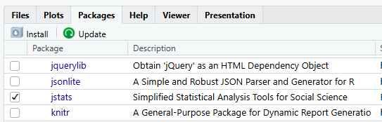
On a fresh load, jstats also prints a short version message in the Console; if it was already loaded, the line stays quiet. And if you’d rather never type the line again, R can run it for you at the start of every session — the Loading jstats automatically page shows how.
For a dataset that ships inside a package, base R has one too: data(community) loads it. The difference shows up beyond package data: data() only reaches datasets bundled in packages, while jload() is one loader for everything on this page — package datasets, your saved .rds files, and SPSS, Stata, SAS, Excel, and CSV files (comma-separated values, a plain-text spreadsheet) — with the same one-line call.
2. Objects, the assignment operator, and the Global Environment
Anything you create in R is stored as an object, and objects live in the Global Environment — the workspace RStudio shows you in the Environment tab of the upper-right pane. Here we make two objects of our own, and open a second dataset alongside the first.
## ---- 2. Objects, the assignment operator, and the Global Environment ----

## "Objects" other than data frames can go into the Environment
## The "Assignment Operator" (less-than followed by a dash) is a key
## base R fundamental
## Take the thing on the right and assign it to what's on the left
## Take the Region variable from the community data frame and assign it
## to a new object
## The new object we'll call "MyObject"
MyObject <- community$Region  # base R

## The name on the left is entirely yours to choose, and the thing on the
## right can be anything at all -- here, just the number 5
x <- 5

## You are not limited to one dataset at a time
## Load a second package dataset, clinic, alongside community
jload("clinic")ConsoleTerminal×Background Jobs×> MyObject <- community$Region # base R > x <- 5 > jload("clinic") Loaded the jstats example dataset 'clinic' 4 variables have SPSS-style missing values: Stress: -99 ["Refused"], -98 ["Don't know"] SleepHours: -99 ["Refused"], -98 ["Don't know"] Medication: -99 ["Refused"] Anxiety4: -99 ["Refused"], -98 ["Don't know"] Missing-value codes detected: MoodRating: -99 (4), -98 (3) Anxiety2: -99 (3), -98 (3) These codes match the missing.convention.codes setting (-99, -98, -97) but are not formally declared, so they are not treated as missing. Declare them as missing if they are; leave as-is if real. No missing-value convention is selected, so these codes cannot be declared yet. Choose one for this session: joptions(missing.convention = "stata") Lowercase markers behave as true NAs in base R. Recommended if you also run base R or AI-generated code. joptions(missing.convention = "spss") Codes stay visible numbers; jstats treats them as missing. Base R does not. joptions(missing.convention = "sas") Like Stata, with uppercase markers (.A-.Z). To make the choice permanent, put the same line in your .Rprofile. Then, to declare one variable's codes as missing: jdeclare_missing(clinic, MoodRating, codes = c(-99, -98), modify = TRUE) To declare and label them in one call, replacing the placeholder names: jdeclare_missing(clinic, MoodRating, codes = c("label1" = -99, "label2" = -98), modify = TRUE) > |
The Global Environment has no real SPSS counterpart, and that is the most useful thing to know about it. In SPSS everything lives inside a dataset: COMPUTE x = 5. does not create an object called x — it adds a column of 5s, one value per case, to whatever dataset is active. There is nowhere for a single value, or a single variable, to sit on its own. (SPSS macros come closest, and hardly anyone uses them.) In R the Environment is exactly that place: a workspace holding objects of any shape, and a data frame is simply one of the shapes.
SPSS can have several datasets open too — but each opens in its own Data Editor window, and switching the active one takes a syntax chain most users never bother with:
GET FILE='community.sav'.
DATASET NAME community.
GET FILE='clinic.sav'.
DATASET NAME clinic.
DATASET ACTIVATE community.
In R there are no windows to juggle: the Environment holds several data frames side by side, and every command simply names the one it uses — the $ in community$Region means “the Region column, in the community dataset.”
3. Cleaning up
Objects you no longer need can be removed, and there are two ways to do it. rm() takes out exactly what you name and leaves everything else alone — which is what you want when one object is wrong and the others are fine. The broom in the Environment pane’s toolbar takes out everything, in one click; RStudio asks you to confirm before it does. The code below uses rm(); the red arrow in the box points out the broom.
One thing to expect: rm() says nothing at all when it works. Silence is success — the Environment pane is where you check.
## ---- 3. Cleaning up ----------------------------------------------------

## Remove MyObject from the Environment
## Note that this is a base R function (j is not the first letter)
rm(MyObject)  # base R

## Remove x as well
rm(x)

## Remove the community data frame
rm(community)

## Remove the clinic data frame
rm(clinic)ConsoleTerminal×Background Jobs×> rm(MyObject) # base R > rm(x) > rm(community) > rm(clinic) > |
The red arrow points to the broom – RStudio calls it Clear objects from the workspace. It empties the Global Environment in one go, which is the button form of the rm(list = ls()) line you will meet later on this page.
When you have finished with a dataset in SPSS you close its Data Editor window, or run DATASET CLOSE clinic. — rm() is the R counterpart. The difference is that the Environment holds more than datasets, so rm() removes any object you name, whatever its shape.
A habit worth starting now: keep your variables inside their data frame. MyObject in block 2 was a copy of one column, community$Region, made only to show what the Environment holds — which is why block 3 removed it. When you work, name the data frame in the call rather than copying a column out on its own, and if you ever build a data frame from separate pieces, check it, then rm() the pieces. jstats works the same way: it analyzes the variables of a data frame. A single vector can be described with jdesc(), jfreq() or jscreen(); anything else is added to the data frame first.
4. How much output you see
jstats can show more or less detail. The output level controls how much appears — so with the Environment empty, load community again and watch it say less.
## ---- 4. How much output you see ----------------------------------------

## The output level is set to "standard" by default
## After you learn more about jstats (and R) you might not want all of
## that output
joutput("minimal")

## With minimal output, you get less information
jload("community")

## Set the output level back to standard
joutput("standard")ConsoleTerminal×Background Jobs×> joutput("minimal") Output Settings Level: minimal effect.size: OFF regression.ci: OFF means.ci: OFF posthoc: OFF diagnostics: OFF case.processing: OFF case.processing.detail: NONE case.processing.filter: COLLAPSE variable.id: NAMES value.id: LABELS ref.categories: OFF model.layout: COEFFICIENTS missing.notice: OFF digits: 3 > jload("community") Loaded the jstats example dataset 'community' > joutput("standard") Output Settings Level: standard effect.size: ON regression.ci: OFF means.ci: ON posthoc: OFF diagnostics: OFF case.processing: AUTO case.processing.detail: TOTALS case.processing.filter: AUTO variable.id: NAMES value.id: BOTH ref.categories: ON model.layout: COEFFICIENTS missing.notice: ON digits: 3 > |
There isn’t one: base R has no output-level setting — each function prints whatever it prints, and how much you see varies with each package author’s choices. joutput() is a single, jstats-wide control.
5. Functions with no arguments, and getting help
Most functions need something inside the parentheses, but a few work on their own. Every function also has a help page.
## ---- 5. Functions with no arguments, and getting help ------------------

## A few functions work correctly without input between the parentheses,
## but most require input
jload()  # This will cause an error with a message about how you might fix the error

## But this one will show you the current output settings for jstats
joutput()

## Here's a base R function that works without arguments/input
## List the objects/data frames in the Environment
ls()  # base R

## Here's another one from base R
## A working directory is the "path" to where your project is stored
## on your computer
## If you're not working in a project, you have to set this yourself (finicky)
getwd()  # base R

## The technical name for a function's inputs are "Arguments"
## View help files describing necessary and optional Arguments by running...
?jload

## The same ? help works for base R functions and functions from any
## installed package
?ls

## And this one opens the package overview: every jstats function,
## grouped by purpose
?jstatsA path is a folder’s address on your computer — the folders you would click through, written out on one line. Three spelling quirks are worth thirty seconds each, because you will meet all three on this page.
The ~ shorthand. Look at the top of your Console: RStudio shows your working directory with a squiggle, something like ~/your-working-directory/. The ~ is shorthand for your home folder (on Windows, usually your Documents folder). getwd() prints that same address written out in full — beginning, on Windows, with a drive letter such as C: or E: that names the disk. Short spelling in the Console header, long spelling from getwd(). Same place.
An address written out from the drive like that is an absolute path: it means the same place whatever folder you are working in. A relative path starts from your working directory instead — "Data/MyData_r.rds" means the file MyData_r.rds in the Data folder inside your project, wherever the project itself sits.
You have met that squiggle before, on the Quick Start page, doing a completely different job — writing a model, as in jt(Optimism ~ Gender). In a file path it has nothing to do with models. Same character, two unrelated jobs.
The slashes. R writes paths with forward slashes (/) on every kind of computer. Windows itself writes the same address with backslashes: File Explorer shows E:\00 R Projects, R shows E:/00 R Projects. Same folder, two spellings. When you type a path in R, use /.
So: ~ means home, / goes between folders, and getwd() tells you the full address of where you are working.
And if all of that felt like a lot, don’t worry. You will not have to type a path anywhere on this page. As long as you work inside an RStudio Project — which is what Before you start asks of you — jstats handles the addresses for you. In a moment you will name a folder once, with joptions(data.dir = "Data"), and jstats creates it inside your project; from then on you load and save with plain file names like "MyData_r.rds", and jstats works out where they belong. Paths are worth recognizing when a message prints one. They are not something you need to write.
? is base R — ?jload, ?ls, and ?mean all work the same way, for base functions and for functions from any installed package. (In RStudio, putting the cursor on a function name and pressing F1 does the same thing. On Macs the key varies from machine to machine — F1 on some, fn + F1 on others, and on some Macs the function keys must first be enabled in System Settings.) What a base R setup doesn’t have is a grouped index: a typical workflow spans functions scattered across many packages, each with its own alphabetical help listing. ?jstats shows the whole toolkit on one page, organized by purpose — one advantage of the functions traveling together as a package.
6. The overwrite prompt
When you load a dataset that’s already open, jstats checks with you before overwriting it — watch for the y/n prompt in the Console window.
## ---- 6. The overwrite prompt -------------------------------------------

## The output you get in the Console Pane can include a confirmation prompt
## Here, jstats will not overwrite community unless you give it permission
jload("community") # Look at the y/n prompt in the console

## Set an optional overwrite argument/input to overwrite without the prompt
jload("community", overwrite = TRUE)The overwrite argument is here to show you two things:
- What an argument looks like. Options go inside the parentheses as
name = value— here,overwrite = TRUE. - Prompts can be overridden. The few times jstats asks for confirmation, the prompt appears in the Console — and each one can be switched off with the right argument. That matters when code runs automatically, with nobody at the keyboard to answer: it happens in several places behind this website, and in the finished script you can download at the bottom of this page.
On its own, base R doesn’t ask. Loading or assigning over an existing object replaces it silently — no prompt, no warning, and the old copy is gone. The confirmation prompt is a jstats safeguard.
7. Saving to a Data folder
Let’s save your work — first with no folder specified, to see where files go by default, and then to a Data folder of your own.
## ---- 7. Saving to a Data folder ----------------------------------------

## Use the assignment operator to copy community to a new data frame
## called MyData
MyData <- community

## Save it with no folder specified -- where does the file go?
## The console message shows the full path: it landed in your project's
## working directory, the default location
## It's the same path the base R getwd() command showed you earlier
jsave(MyData, "WhereDidIGo.rds")

## Delete that test file
## file.remove() is base R -- the file-on-disk equivalent of the rm()
## you used for data frames. It replies with a cryptic [1] TRUE
file.remove("WhereDidIGo.rds")  # base R

## Now name a Data folder of your own
## jstats creates the folder right away (if it isn't already there)
joptions(data.dir = "Data")

## Save the dataset to the Data folder and call it MyData_r.rds
## Specify R format with the .rds extension
jsave(MyData, "MyData_r.rds")
Where these messages read ~/your-working-directory/, your own screen shows the real name of your project folder – the same one the Console header names, just above.
ConsoleTerminal×Background Jobs×> MyData <- community
> jsave(MyData, "WhereDidIGo.rds")
Saved MyData to ~/your-working-directory/WhereDidIGo.rds
(R format; 103 cases, 15 variables)
> file.remove("WhereDidIGo.rds")  # base R
[1] TRUE
> joptions(data.dir = "Data")
Options Settings
Data folder: Data
Run joptions() to see all settings.

Created 'Data' folder in working directory.

> jsave(MyData, "MyData_r.rds")
Saved MyData to ~/your-working-directory/Data/MyData_r.rds
(R format; 103 cases, 15 variables)
> |
The Files pane (lower right) is where the new Data folder appears – alongside whatever else your project folder already holds. Click the folder's name there and you'll find MyData_r.rds inside.
Why set a data folder at all? Tidiness now, and a payoff later. With data.dir set, every save and load on this page knows where to look. And that’s the habit to keep: put joptions(data.dir = "Data") near the top of your own scripts — or, once, in your Project’s .Rprofile, so every session in that Project starts with it already set (Loading jstats and its options automatically shows how). Then drop a dataset of yours into that folder and jload("YourFile.sav") opens it by name alone. If you’re not sure where the folder is on your computer, the jsave message has already told you — it prints the full path each time, ready to paste into File Explorer (Windows) or find in Finder (Mac).
Saving to the working directory by default is base R’s behavior too — saveRDS(MyData, "MyData_r.rds") puts the file in the same place; jstats just tells you, in full, where it went. To use a folder, base R won’t create it for you (that’s dir.create("Data") first), and the folder name gets typed into every path from then on — with any subfolders along for the ride, e.g. saveRDS(MyData, "Data/CommunityStudy/Wave1/MyData_r.rds"). joptions(data.dir = ...) sets the location once, and every jsave() and jload() after that already knows where to look.
And note what file.remove() didn’t do: ask. Like the silent overwrite in block 6, base R deletes with no confirmation — mix up a filename and a real data file is gone. jstats’s prompts exist precisely because of edges like that.
8. Gone from the Environment
You have just saved MyData to a file on disk. Now remove it — and community — from the Environment. Before you run the block, make a prediction: is the file you just saved gone as well?
## ---- 8. Gone from the Environment --------------------------------------

## Remove both data frames from the Environment
## What happens to the file you just saved? The next block finds out
rm(MyData)  # base R
rm(community)ConsoleTerminal×Background Jobs×> rm(MyData) # base R > rm(community) > |
9. Getting it back, and saving across formats
There it is. The Environment is temporary; the file on disk is not. Load it straight back — then send it out to other formats, where one wrinkle around missing values needs handling, and jstats handles it for you.
## ---- 9. Getting it back, and saving across formats ---------------------

## The file survived: jload() brings the saved dataset straight back
jload("MyData_r.rds")

## The original community dataset carries SPSS-style missing values
## So it saves to SPSS format (.sav) without a problem
jsave(MyData_r, "MyData_spss.sav")

## But the SPSS-style missing-value codes need to be converted
## if you want to save to a format other than R or SPSS
jsave(MyData_r, "MyData_stata.dta")  # This will draw an error

## Convert to Stata format (.dta)
MyData_stata <- jconvert(MyData_r, to = "stata")
jsave(MyData_stata, "MyData_stata.dta") # Now no errorConsoleTerminal×Background Jobs×> jload("MyData_r.rds") Reading from ~/your-working-directory/Data Loaded MyData_r (R format; 103 cases, 15 variables) 5 variables have SPSS-style missing values: Income: -99 ["Refused"], -98 ["Don't know"] Education: -99 ["Refused"], -98 ["Don't know"] Smoker: -99 ["Refused"] Environment1: -99 ["Refused"], -98 ["Don't know"] Environment3: -99 ["Refused"], -98 ["Don't know"] > jsave(MyData_r, "MyData_spss.sav") Saved MyData_r to ~/your-working-directory/Data/MyData_spss.sav (SPSS format; 103 cases, 15 variables) > jsave(MyData_r, "MyData_stata.dta") # This will draw an error Error: jsave(): 5 variables carry SPSS-style missing values, incompatible with the .dta format: Income, Education, Smoker, Environment1, Environment3 Before saving to Stata format, convert with: jconvert(MyData_r, to = "stata", modify = TRUE) Or save every declared missing value as plain NA instead: jsave(MyData_r, "MyData_stata.dta", preserve.declarations = FALSE) > MyData_stata <- jconvert(MyData_r, to = "stata") Converted to Stata-style missing values in 5 variables: Income -99 ["Refused"] -> .a -98 ["Don't know"] -> .b Education -99 ["Refused"] -> .a -98 ["Don't know"] -> .b Smoker -99 ["Refused"] -> .a Environment1 -99 ["Refused"] -> .a -98 ["Don't know"] -> .b Environment3 -99 ["Refused"] -> .a -98 ["Don't know"] -> .b This call changes MyData_r only if you assign the result: MyData_r <- jconvert(MyData_r, ...) To change MyData_r directly, rerun with modify = TRUE: jconvert(MyData_r, ..., modify = TRUE) > jsave(MyData_stata, "MyData_stata.dta") # Now no error Saved MyData_stata to ~/your-working-directory/Data/MyData_stata.dta (Stata format; 103 cases, 15 variables) > |
In SPSS, user-missing values are declared in Variable View and travel with the file. When you Save As a different format, those definitions don’t always carry across cleanly. jstats keeps the equivalent information with your data, and when a format needs it in a different form, jconvert() does the translation — which is why saving straight to Stata format above stops and offers two ways forward: convert first, or save every declared missing value as a plain NA.
By itself, base R can’t write SPSS, Stata, or SAS files. You’d install and load the haven package and call haven::write_sav(), haven::write_dta(), or haven::write_xpt() yourself — and haven is exactly the proven package jstats uses under the hood, so nothing here reinvents the wheel. What jstats spares you is the setup and the sharp edge: loading an extra package in every script, learning its separate function set, and handling the missing-value translation by hand — haven refuses SPSS-style missing codes headed into Stata format, just as you saw above, and converting them yourself is genuinely fiddly. jconvert() is that translation, done for you.
Two conversion habits are worth knowing even if you’re an experienced R user.
10. Reloading, and how missing codes travel
Load the saved files back and see how each format keeps its missing-value codes.
## ---- 10. Reloading, and how missing codes travel -----------------------

## You removed data frames one at a time earlier; this clears them all at once
## It is the code equivalent of the broom button in the Environment pane
rm(list = ls())  # base R

## Load all data sets back
jload("MyData_r.rds")
jload("MyData_spss.sav")
jload("MyData_stata.dta")

## Examine how the missing codes are kept in the different formats
jfreq(MyData_r, Education)  # will print whatever was originally stored
jfreq(MyData_spss, Education)  # SPSS-style declared missing codes
jfreq(MyData_stata, Education) # Stata-style declared missing codes

MyData_r_stata <- jconvert(MyData_r, to = "stata")
jfreq(MyData_r_stata, Education) # Now the codes display in Stata formatConsoleTerminal×Background Jobs×> rm(list = ls()) # base R > jload("MyData_r.rds") Reading from ~/your-working-directory/Data Loaded MyData_r (R format; 103 cases, 15 variables) 5 variables have SPSS-style missing values: Income: -99 ["Refused"], -98 ["Don't know"] Education: -99 ["Refused"], -98 ["Don't know"] Smoker: -99 ["Refused"] Environment1: -99 ["Refused"], -98 ["Don't know"] Environment3: -99 ["Refused"], -98 ["Don't know"] > jload("MyData_spss.sav") Reading from ~/your-working-directory/Data Loaded MyData_spss (SPSS format; 103 cases, 15 variables) 5 variables have SPSS-style missing values: Income: -99 ["Refused"], -98 ["Don't know"] Education: -99 ["Refused"], -98 ["Don't know"] Smoker: -99 ["Refused"] Environment1: -99 ["Refused"], -98 ["Don't know"] Environment3: -99 ["Refused"], -98 ["Don't know"] > jload("MyData_stata.dta") Reading from ~/your-working-directory/Data Loaded MyData_stata (Stata format; 103 cases, 15 variables) 5 variables have Stata-style missing values: Income: .a ["Refused"], .b ["Don't know"] Education: .a ["Refused"], .b ["Don't know"] Smoker: .a ["Refused"] Environment1: .a ["Refused"], .b ["Don't know"] Environment3: .a ["Refused"], .b ["Don't know"] > jfreq(MyData_r, Education) # will print whatever was originally stored Frequencies 103 Cases in the 1 Variable Pool Education Freq Total % Valid % Cum. % ----------------------- ---- ------- ------- ------ Valid 1: Some high school 23 22.33 23.71 23.71 2: High school graduate 18 17.48 18.56 42.27 3: Some college 25 24.27 25.77 68.04 4: Bachelor's degree 13 12.62 13.40 81.44 5: Graduate degree 18 17.48 18.56 100.00 Total valid 97 94.17 100.00 Missing -99 ["Refused"] 3 2.91 -- -- -98 ["Don't know"] 3 2.91 -- -- Total missing 6 5.83 Total 103 100.00 > jfreq(MyData_spss, Education) # SPSS-style declared missing codes Frequencies 103 Cases in the 1 Variable Pool Education Freq Total % Valid % Cum. % ----------------------- ---- ------- ------- ------ Valid 1: Some high school 23 22.33 23.71 23.71 2: High school graduate 18 17.48 18.56 42.27 3: Some college 25 24.27 25.77 68.04 4: Bachelor's degree 13 12.62 13.40 81.44 5: Graduate degree 18 17.48 18.56 100.00 Total valid 97 94.17 100.00 Missing -99 ["Refused"] 3 2.91 -- -- -98 ["Don't know"] 3 2.91 -- -- Total missing 6 5.83 Total 103 100.00 > jfreq(MyData_stata, Education) # Stata-style declared missing codes Frequencies 103 Cases in the 1 Variable Pool Education Freq Total % Valid % Cum. % ----------------------- ---- ------- ------- ------ Valid 1: Some high school 23 22.33 23.71 23.71 2: High school graduate 18 17.48 18.56 42.27 3: Some college 25 24.27 25.77 68.04 4: Bachelor's degree 13 12.62 13.40 81.44 5: Graduate degree 18 17.48 18.56 100.00 Total valid 97 94.17 100.00 Missing .a ["Refused"] 3 2.91 -- -- .b ["Don't know"] 3 2.91 -- -- Total missing 6 5.83 Total 103 100.00 > MyData_r_stata <- jconvert(MyData_r, to = "stata") Converted to Stata-style missing values in 5 variables: Income -99 ["Refused"] -> .a -98 ["Don't know"] -> .b Education -99 ["Refused"] -> .a -98 ["Don't know"] -> .b Smoker -99 ["Refused"] -> .a Environment1 -99 ["Refused"] -> .a -98 ["Don't know"] -> .b Environment3 -99 ["Refused"] -> .a -98 ["Don't know"] -> .b This call changes MyData_r only if you assign the result: MyData_r <- jconvert(MyData_r, ...) To change MyData_r directly, rerun with modify = TRUE: jconvert(MyData_r, ..., modify = TRUE) > jfreq(MyData_r_stata, Education) # Now the codes display in Stata format Frequencies 103 Cases in the 1 Variable Pool Education Freq Total % Valid % Cum. % ----------------------- ---- ------- ------- ------ Valid 1: Some high school 23 22.33 23.71 23.71 2: High school graduate 18 17.48 18.56 42.27 3: Some college 25 24.27 25.77 68.04 4: Bachelor's degree 13 12.62 13.40 81.44 5: Graduate degree 18 17.48 18.56 100.00 Total valid 97 94.17 100.00 Missing .a ["Refused"] 3 2.91 -- -- .b ["Don't know"] 3 2.91 -- -- Total missing 6 5.83 Total 103 100.00 > |
11. Turning up the digits
One more control before the final check: how many decimal places jstats shows. The default setting is 3, the maximum is 7 — and for what comes next, we want all 7. (Not everything follows the setting: p-values keep their own three decimals, percentages their one, and counts and a variable’s minimum and maximum print as they are.)
## ---- 11. Turning up the digits -----------------------------------------

## By default, jstats shows 3 decimal places
jdesc(MyData_r, Age)   # see the Age mean below -- the callouts explain the decimals

## Turn the display up to the maximum of 7 decimal places
joutput(digits = 7)
jdesc(MyData_r, Age) # the same mean, now with more decimals shownConsoleTerminal×Background Jobs×> jdesc(MyData_r, Age) # see the Age mean below -- the callouts explain the decimals Descriptive Statistics 103 Cases in the 1 Variable Pool Variable Total Non_missing Min Max Mean SD -------- ----- ----------- --- --- ------ ------ Age 103 103 18 71 40.650 11.620 > joutput(digits = 7) Output Settings digits: 7 (override) Run joutput() to see all settings. > jdesc(MyData_r, Age) # the same mean, now with more decimals shown Descriptive Statistics 103 Cases in the 1 Variable Pool Variable Total Non_missing Min Max Mean SD -------- ----- ----------- --- --- ---------- ---------- Age 103 103 18 71 40.6504854 11.6195480 > |
jstats prints every statistic to the number of decimal places digits asks for, zeros included — so the mean above reads 40.650 at the default setting of 3, the way an SPSS table would pad it. Stata’s default display format goes the other way and drops trailing zeros. Counts, and the Min and Max (values from the data, not statistics), print as they are at any setting.
The closest is options(digits = ...), and it’s a different animal: it sets significant digits, globally, for nearly everything R prints. joutput(digits = ...) means decimal places, and it changes only jstats output.
12. The proof that nothing was lost
Those three data frames each made a round trip through a different file format. If the trips were truly lossless, the same statistics should come back from every one of them — right down to the seventh decimal.
## ---- 12. The proof that nothing was lost -------------------------------

## Ask for the mean of Age from each of the three reloaded data frames
jdesc(MyData_r, Age)
jdesc(MyData_spss, Age)
jdesc(MyData_stata, Age)
## All three report the identical mean, to the last decimal:
## same data, three file formats, nothing lost along the way

## And one base R caution, shown live (the box below explains):
## Income carries declared missing-value codes (-99, -98)
jdesc(MyData_spss, Income)   # the correct mean -- jdesc leaves the codes out
## Now ask base R's mean() for the same column. It knows nothing about the
## declarations, so the -99s and -98s go straight into the average
mean(MyData_spss$Income)  # base R -- a poisoned mean

## Set the display back to the default before you go
joutput(digits = 3)

## Put the data folder setting back to its default (the working directory) too
## NULL clears the setting
## A finished script leaves your session exactly as it found it
joptions(data.dir = NULL)ConsoleTerminal×Background Jobs×> jdesc(MyData_r, Age) Descriptive Statistics 103 Cases in the 1 Variable Pool Variable Total Non_missing Min Max Mean SD -------- ----- ----------- --- --- ---------- ---------- Age 103 103 18 71 40.6504854 11.6195480 > jdesc(MyData_spss, Age) Descriptive Statistics 103 Cases in the 1 Variable Pool Variable Total Non_missing Min Max Mean SD -------- ----- ----------- --- --- ---------- ---------- Age 103 103 18 71 40.6504854 11.6195480 > jdesc(MyData_stata, Age) Descriptive Statistics 103 Cases in the 1 Variable Pool Variable Total Non_missing Min Max Mean SD -------- ----- ----------- --- --- ---------- ---------- Age 103 103 18 71 40.6504854 11.6195480 > jdesc(MyData_spss, Income) # the correct mean -- jdesc leaves the codes out Descriptive Statistics 103 Cases in the 1 Variable Pool Variable Total Non_missing Min Max Mean SD -------- ----- ----------- ----- ----- ------------- ------------- Income 103 97 14000 93000 49855.6701031 17427.2234896 > mean(MyData_spss$Income) # base R -- a poisoned mean [1] 46945.72 > joutput(digits = 3) Output Settings digits: 3 Run joutput() to see all settings. > joptions(data.dir = NULL) Options Settings Data folder: Working directory Run joptions() to see all settings. > |
jdesc() is the counterpart of SPSS’s Analyze > Descriptive Statistics > Descriptives — the same N, minimum, maximum, mean, and standard deviation you’d read from that output table. And the check above may feel familiar from practice: reopening a dataset that’s been through another format, and confirming the descriptives still match.
The matching numbers are only half the story — the missing-value declarations made the round trip too, which is arguably the bigger deal. You saw it back in block 10: Education’s codes come through meaning the same thing in every file, with the Stata copy simply wearing its .a/.b form. In SPSS terms, your MISSING VALUES definitions survived the Save As.
One thing that may differ on your screen: if you have chosen a missing-value convention — on Telling jstats about missing values, or in your Project’s .Rprofile — jstats notices when a file arrives in a different form and adds a line to the load message saying so. That extra line is the setting working, not a problem with the file. (Age itself carries no missing codes — that’s exactly why it makes a clean test variable here.)
For a clean variable like Age, base R agrees exactly: mean(MyData_r$Age) returns the same 40.65049. The difference appears with variables that carry declared missing-value codes, like Income — those codes are ordinary numbers to base R, and the block’s last lines show the damage live: mean(MyData_spss$Income) folds the -99s and -98s straight into the average, while jdesc() reads the declarations and leaves the codes out automatically — provided the declarations exist: here they traveled with the files, and when a dataset arrives with codes that were never declared, you add the declarations yourself with jstats’s jdeclare_missing() function — Telling jstats about missing values walks that through live. It’s the same protection you’d expect from commercial statistical software.
The download at the bottom of this page is the finished version of what you built — and finished means something specific. A goal every experienced programmer and statistician takes for granted, but new researchers are rarely told: a completed script should run from beginning to end without errors. On this page you experimented — deliberate errors and prompts included, because that’s how working scripts develop. The download shows what the end of that process looks like, and it differs from the page blocks in three principled ways: the deliberate error lines are commented out, the y/n prompt line is commented out (a prompt would pause an unattended run), and the saves — plus the one reload that could collide with an earlier run’s leftovers — carry overwrite = TRUE so the whole file can be run again and again, exactly the automatic-execution override from block 6.
To prove a script is finished, use the Source icon (to the right of Run in the script toolbar): it runs the entire file, top to bottom, in one go. A few things to know. Source shows the output without echoing each command back to the Console — that’s normal — and the small arrow beside Source offers “Source with Echo” if you’d like the commands shown too. jstats functions print their own tables, so their output always appears; but a bare base R line that merely displays a value — ls(), getwd(), mean() — stays quiet under Source, because R only auto-prints results when you run lines interactively — and even interactively, what it prints is a bare, unlabeled number. And if you re-run the script you pasted together yourself, the saves will refuse to overwrite their earlier files — that’s block 6’s lesson again; add overwrite = TRUE just as the finished file does.
The What you should see boxes under some blocks above reproduce that Console — the blue command lines, the gray notices, the colored tables, a red error where one is meant to happen. They show the code being run, along with any note written on the end of a command line — but not the standalone ## comment lines (running one just echoes it back and does nothing), so the box stays focused on what actually happens. Reading a block? The commented code is in the gray block; the result is in the box beneath it. Several boxes also picture your Environment pane — the upper-right one — so you can watch objects appear and disappear as you work. And where a file path appears, the boxes print ~/your-working-directory/ in place of a real folder name: on your own screen that reads as the actual path to your project.
Nothing needs deleting between runs, and nothing is deleted: the overwrite arguments handle the repeats, and the Data folder with its three saved files stays put after every run — that’s what saving is for. Remove the files by hand if you ever want a clean slate.
One more setup idea if you’re keeping the file — and it’s worth keeping: finished scripts travel. Sooner or later you’ll share one with a collaborator, or receive one from someone else, and a script that runs top to bottom on another person’s computer is the standard to aim for. So a downloaded script deserves a proper home: jstats created the Data folder for you during the run-through, but you can also make folders yourself in RStudio — in the Files tab of the lower-right pane, click New Folder and type a name into the popup. “Scripts” is a good one for storing this download, and it will appear right beside the Data folder you created by following the steps above.
Take the whole script with you
That’s the full run-through. If you’d like the entire script in one file to keep, adjust, and reuse, download it here:
The file is close to what you have just built: the same code, in the same order, as though you had pasted every block above into one script. Three things differ, each on purpose — the lines that raise a deliberate error are commented out, the line that triggers the y/n prompt is commented out (a prompt would stall a script left to run on its own), and the saves carry overwrite = TRUE so the whole file can be run again and again. The What’s the point? box under the last block explains why a finished script is written that way.